This is the final iteration of the algorithm. It took many ideas and evaluations to reach this stage, some of which weren’t documented, and others that fortunately were. If you’re interested in precursors to the ideas discussed here, read about our first and second iterations.
Summary
The algorithm is composed of multiple layers—and effectively, multiple components—where each layer has a distinct purpose. Each layer takes its input from a dedicated storage component and stores its output in another dedicated storage component. The reports roughly “flow” through the system as follows:
- The event matcher matches up any two reports that are within a set time tolerance (e.g. 5 minutes) and occurred at the same TIPLOC. It then passes on these event matchings onto the service matcher.
- The service matcher takes the event matchings and creates new service matchings and updates existing ones. (A single service matching is composed of a service, a unit and some properties between their matched events, like mean time difference.) The service matcher does no filtering—if there is a single event matching corresponding to a single service and a unit, a service matching is produced. The event matchings are discarded after each run of the service matcher, but service matchings persist on the database.
- Since the service matcher does no filtering, there are lots of improbable service matchings created. The matchings component takes service matchings from the database and filters the most likely matchings for every unit. This is where the decision on what a good matching is made, based on:
- the properties of a service matching, calculated by the service matcher
- the (genius) allocations given, as part of the extract
Detailed Explanation
Simulator
The simulator is responsible for simulating a real-time environment for the algorithm. It gets reports from the extract, which is stored in the database, and passes the reports onto the event matcher. It always gets and processes whatever the next report is, so effectively “simulated time” is not linear but is dictated by the “spacing” between reports. This way, the algorithm runs and terminates as quickly as it possibly can, allowing us to better estimate performance.
TRUST and GPS reports are represented as Python dictionaries, parsed from and containing all the original fields of the extract:
TRUST
{
  'id': Integer, # a unique ID, generated by the system
  'headcode': String,
  'origin_location': String,
  'origin_departure': DateTime,
  'tiploc': String,
  'seq': Integer,
  'event_type': String,
  'event_time': DateTime,
  'planned_pass': Boolean
}
GPS
{
  'id': Integer, # a unique ID, generated by the system
  'gps_car_id': String,
  'event_type': String,
  'tiploc': String,
  'event_time': DateTime
}
Event matcher
The event matcher is the first layer of the algorithm. It’s the component that the reports are passed onto to be processed and its task is to match up TRUST and GPS reports that occurred at the same TIPLOC within 5 minutes of each other. It does this by keeping 30 minute caches of the latest TRUST and GPS reports that occurred at every TIPLOC. Additionally, the event matcher also updates the tracker, which holds some statistics about services and units for quick access.
Caches
To match up reports, the event matcher keeps 2 caches—one of TRUST and one of GPS reports. The caches are optimized to hold time-limited data, indexed by TIPLOC.
In our prototype, the cache uses a Python dictionary, with TIPLOC as key and a list of sorted reports as value.
Tracker
For each service and unit, the tracker keeps track of:
- The identifiers for all the services and units that were “seen”
- The total number of reports from each service/unit
- The times of the first and last reports received for each service/unit
This data is used at a later stage, when services are matched with units.
Queue
The event matcher passes on matching reports to the queue. The queue stores an event matching as a dictionary, like so:
Event matching
{
  'trust_id': Integer,
  'gps_id': Integer,
  'trust_event_time': DateTime,
  'gps_event_time': DateTime
}
The ids are kept to test for uniqueness later, and the event times to calculate the mean time error.
Event matchings are stored in lists, depending on the service and unit it belongs to, and the whole data structure is a Python dictionary which has “service matching keys”, which are Python tuples:
Service matching key
(headcode, origin_location, origin_departure, gps_car_id)
The first 3 values essentially represent a service and come from the TRUST report, whereas the last represents a unit and comes from the GPS report. The complete data structure looks like:
{
  [service matching key]: [
    [event matching],
    [event matching],
    [event matching],
    ...
  ],
  [service matching key]: [
    ...
  ]
}
The queue is emptied whenever the event matchings are retrieved.
Service matcher
From the queue, the reports are passed onto the service matcher. The service matcher runs periodically (15 minutes in our prototype) and processes all event matchings that are in the queue. For every service matching key in the queue, the service matcher either updates the service matching (if it exists in the database) or creates a new service matching. Once it finishes, it notifies the matchings component with the keys of the service matchings that have changed.
Service matchings are stored in the database, but the database rows are represented as equivalent Python dictionaries while being manipulated. Below is the structure of a service matching:
Service matching
{
  'headcode': String,
  'origin_location': String,
  'origin_departure': DateTime,
  'gps_car_id': String,
  'mean_time_error': Float, # in minutes
  'variance_time_error': Float, # in minutes^2
  'total_matching': Integer,
  'start': DateTime,
  'end': DateTime
}
- The
headcode,origin_location,origin_departureandgps_car_idcome from the service matching key, which as we mentioned, is stored in the queue. - A time error is considered the time difference between matched TRUST and GPS reports. The
mean_time_erroris the mean of time errors of all event matchings for a given service matching key, andvariance_time_errortheir calculated variance. - The
total_matchingfield holds the total number of (unique) TRUST reports that were matched with a GPS report. - The
startandendfields store the start and end times of the service matching.
New service matchings
For new service matchings that don’t exist on the database (or rather, service matchings keys that don’t exist in the database), the fields above are calculated from all the event matchings received from the queue for the given service matching key.
- To calculate
mean_time_error, we use the standard formula:
mean = sum(time_errors) / len(time_errors)
- Likewise for
variance_time_error:
variance = sum((mean - value)**2 for value in time_errors) / len(time_errors)
- To count the
total matchingTRUST reports, we count the total uniquetrust_ids in the event matchings. - The
start/endtimes of the service matching are the earliest/latesttrust_event_timeorgps_event_time(whichever is earliest/latest) in the event matchings.
Existing service matchings
When a service matchings already exists in the database, a new service matching is created from the event matchings in the queue, and fields calculated (as above). The two (existing and new) service matchings are then combined:
headcode,origin_location,origin_departureandgps_car_idare the same in both existing and new service matchings, since they represent the service matching key.mean_time_errorandvariance_time_errorare combined from the two, using Youngs and Cramer updating formulas (adapted from this paper).total_matchingare simply added from the two service matchingsstartis simply the earlieststartof the two service matchings, andendthe latestend.
Matchings
In the final layer, the matchings component filters only the most likely matchings—these will essentially say which unit ran which service. It also keeps and updates a local copy of unit matchings, which are simply all the service matchings that were assigned to a specific unit.
The matchings component stores gets notified by the service matcher about the keys of the service matchings that have changed. Every time the matchings component receives a notification:
- It extracts the unique
gps_car_ids from the changed service matching keys. These are the units for which at least one service matching was changed. For eachgps_car_id, it: - Retrieves all the service matchings in the database that belong to it.
- Filters out service matchings that do not satisfy the minimum matching criteria (more below).
- Assigns a score to each service matching remaining and sorts them by descending score (more below).
- It traverses the sorted list of service matchings and assigns each to the
gps_car_idif it doesn’t overlap (in time) with a previously assigned matching. If it does overlap, it simply ignores it and moves on to the next.
At the end of this process, the unit matchings stored locally are updated, and can be retrieved by an external system (in our case, the visualisation).
Minimum matching criteria
We mentioned that the matchings component filters out service matchings that do not satisfy the minimum matching criteria. These criteria are as follows:
- If a service matching is in the predetermined allocations, then it does satisfy the minimum criteria, regardless of other properties.
- If a service matching is not in the allocations, then it only satisfies the criteria if all of the following are true for the service matching:
- The
total_matchingnumber of reports is greater than 2 - The
variance_time_erroris less than 6.0 - The absolute of the
mean_time_erroris less than 1.5 - If the service has less than 6
total_matchingnumber of reports, then:- its
variance_time_errorneeds to be less than 2 - the absolute of the
mean_time_errorless than 1.0
- its
- If the service matching time length (
end - start) is less than 15 minutes, then it has to match 35% of the total reports of the service
- The
The criteria are all calculated from the fields that are stored in each service matching that we discussed earlier.
Service matching scores
We mentioned that each service matching is given a score. The score is a Python tuple:
Score
(
  close_match,
  total_matching_score,
  error_score,
  matched_over_total_score,
  meets_low_requirements
)
close_matchis a boolean and True only if all of the following are True:total_matchingis greater than 8- the absolute of
mean_time_erroris less than 1.0 variance_time_erroris less than 2.0
total_matching_scoreis an integer that is calculated by taking the integer value oftotal_matching / 5error_scoreis an integer calculated by taking the integer value ofmean_time_error / 0.4matched_over_total_scoreis the integer oftotal_matching / total_for_service. “Total for service” is the total number of reports of the service.meets_low_requirementsis a boolean that is True whenvariance_time_erroris less than 3.0.
Some of the properties above (like total_matching_score and error_score) are meant to place values of certain intervals into “buckets”, so that when sorting, values in the same bucket get equal precedence.
Achievements
Related to the algorithm, the following are our key achievements:
- The algorithm works in real-time, as required by our client.
- The algorithm generates results incrementally—only the part of the result that is affected by the change is recalculated, leaving the rest unchanged.
- With the layered design, the algorithm can operate in 3 separate workers, communicating between layers with data stores.
We also created a visualisation to inspect the matchings and provided it with the final prototype.
System Manual
This part of the manual gives a quick overview of the entire system to understand the underlying structure of the project and how to setup the system.
Technology Stack
In the following image, you can see an outline of our technology stack.
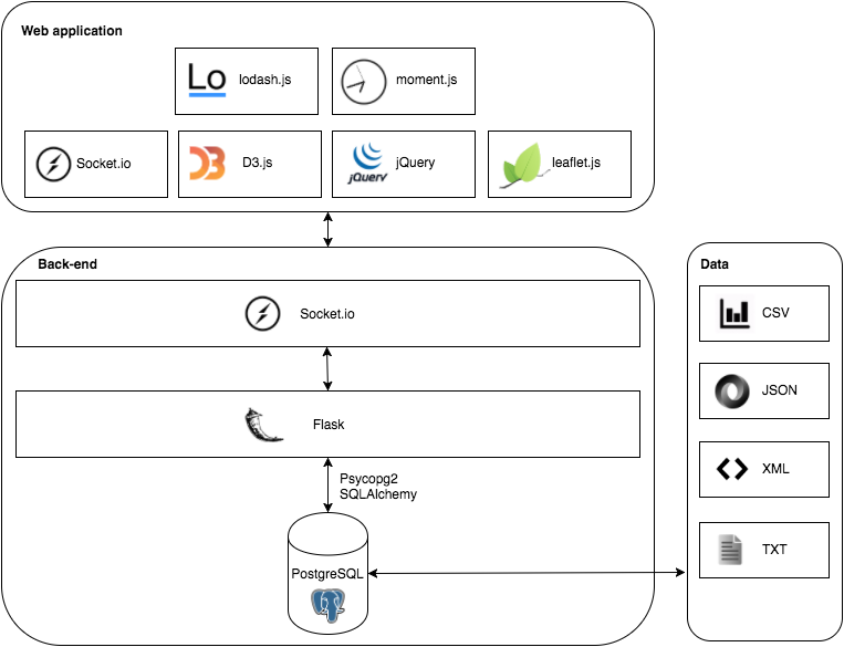
We are using the flask web framework together with a PostgreSQL database. SQLAlchemy and psycopg2 are used to write SQL queries to the database in Python. Finally to provide real-time data to the client, we use Flask-SocketIO.
In the front-end, we also use socket.io to manage the web socket on the client’s side. D3.js and leaflet.js are then used to visualise all of the report matchings. Finally other helper libraries used are: lodash.js, moment.js and jquery.
Most of the data provided came in a variety of formats. First of all, the diagrams are all txt files. The specifications of what specific characters mean can be found here. Most of the other data was in a more comprehensible format such XML (GPS and TRUST reports) and CSV (Unit to GPS mapping and genius allocations).
Setting Up
To get started, you will need to install pip, git, PostgreSQL (and brew, if you’re using a mac).
Setting Up the Database
Create a postgres database with psql (installed with PostgreSQL):
CREATE USER atos WITH PASSWORD 'atos';
CREATE DATABASE atos WITH OWNER atos;
GRANT ALL PRIVILEGES ON DATABASE atos TO atos;
Setting Up a Local Environment
First, you will need to install virtualenv using pip:
pip install virtualenv
After you have virtualenv installed, create a virtual environment:
virtualenv venv
In your new virtual environment, clone the repository and cd into the correct repository
git clone https://github.com/ucl-team-8/service.git service
cd service
Then run these bash commands to set the environment variables in your virtual environment activate file:
echo "export APP_SETTINGS='config.DevelopmentConfig'" >> venv/bin/activate
echo "export DATABASE_URL='postgres://atos:atos@localhost/atos'" >> venv/bin/activate
Activate your virtual environment by running:
source venv/bin/activate
Finally, install all dependencies from requirements.txt:
pip install -r requirements.txt
Installing Visualisation Dependencies
To install node and npm on a Mac, run:
brew install node
If you don’t have brew, see installation instructions here.
To install node and npm on Windows, download it from nodejs.org.
After you have npm, run:
npm install -g jspm
npm install
jspm install
Finally, your local environment should be set up.
Creating the Database Tables
We use Flask-Migrate to handle database migrations. To create the necessary database tables, run:
python manage.py db upgrade
Importing Data
You will first need to get a copy of the locations.tsv file with all of the TIPLOC locations. This file is not publicly available since it is considered confidential information.
To import all of the data in the data directory, either run:
python import/import.py northern_rail
or:
python import/import.py east_coast
depending on which data set you would like to import.
Folder Structure
.
├── algorithm           # Old iteration of the algorithm
├── algorithm2          # Improved version of the algorithm
├── data                # All of the sample data
|   ├── east_coast      # Extract from the east coast
|      └── ...
|   ├── northern_rail    # Extract from northern rail
|      └── ...
|   ├── locations.tsv   # gitignored file with locations of tiplocs
├── import              # Contains the import script to import data into database.
├── migrations          # All of the database generated by alembic
├── static              # The static files for the client
|   ├── css
|   ├── data            # Can be ignored, is used if you want to directly serve a data file to the client
|   ├── images
|   ├── js
|      ├── live         # All of the code for the prototype application on client.
|         ├── map       # Uses D3 and leaflet to visualise matching on a map
|         ├── reports   # Renders the reports next to the map
|         ├── services  # Shows all of the services and search
|         ├── utils     # All utility functions
|         └── index.js  # Combines all of the functionality
|   └── ...
├── templates           # All of the html templates that can be rendered
├── tests               # Folder with all of the tests for the python code
├── app_socketio.py     # Deals with clients connecting through socketio
├── app.py              # Serves all of the html web pages
├── config.py           # Flask configurations
├── manage.py           # Manages database models and migrations
├── models.py           # All of the database models
├── package.json        # npm dependencies
├── README.md
├── requirements.txt    # Python packages used
└── ...
User Manual
UI
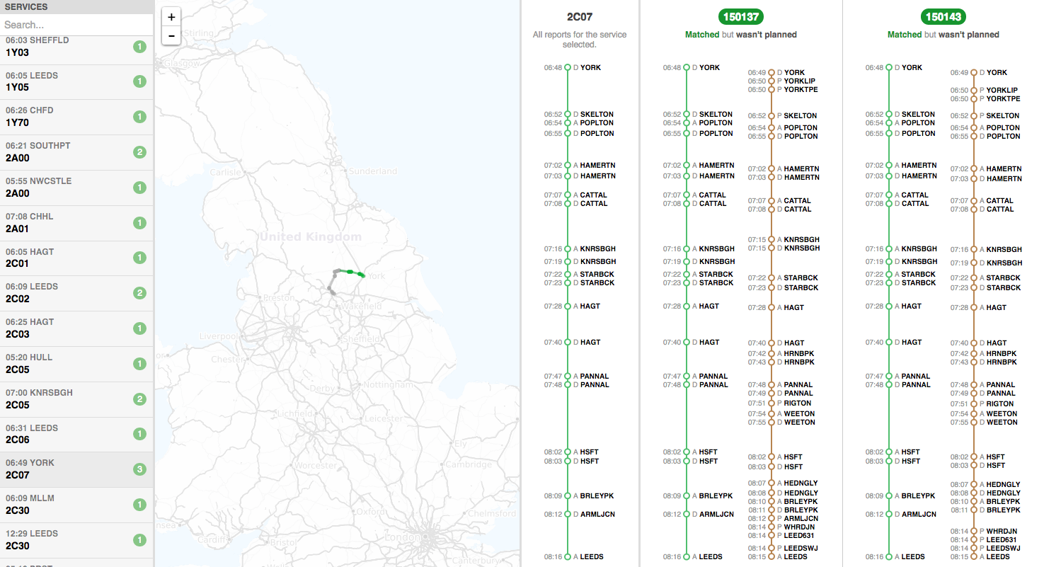
The UI is divided up into three vertical panes.
Left pane
On the left are all the services that the algorithm has seen so far. There are some numbers in coloured circles:
- green is the number of new matchings found that didn’t exist in the allocations
- gray is the number of matchings found that did already exist in the allocations
- red is the number of matchings that did exist in the allocations, but are wrong according to the algorithm
The services that are “interesting” (red and green) are shown first in the list, and the “boring” (gray) are last.
The search field at the top allows searching for:
- a headcode (e.g.
2C07) - a gps_car_id (e.g.
150148), which will find all services for the gps_car_id addedwill find services with green circlesunchangedwill find services with gray circlesremovedwill find services with red circles
Selecting a service will show more information in the middle and right pane.
Middle pane
The middle pane shows a map with:
- TRUST reports of the service in green
- GPS reports of the unit in brown
Only the selected service is plotted by default, but you can plot matchings by moving your mouse over them in the right pane.
You can also zoom by scrolling (or the + and - buttons) and pan by dragging. The current time of the simulation is shown in the top right corner (if the simulation is running).
Right pane
The right pane shows matchings of the selected service with different units.
At the top is the headcode or gps_car_id. If they are shown in green then the algorithm decided that they match, otherwise, if they’re in red, then they do not match, but are planned in the allocations.
Below them are the reports. In green are TRUST reports of the service, and in brown are GPS reports of the unit. The reports are sorted chronologically, with earliest at the top and latest and the bottom.
Moving your mouse over the reports will display on the map the approximate, interpolated location of the service and the unit at that specific time. This helps determine how close they were running, and whether they do indeed match.
Testing and Evaluation
Due to the nature of the problem, the output of the algorithm is very hard to test programmatically. Initially, our plan was to get all of the manual matches and write tests that use results from historic data to verify the accuracy of the algorithm. However, our client warned us that those matchings were still prone to error because they were all made manually. So we decided to use other techniques to test our final solution.
Unit Tests
We wrote unit tests to test almost all individual units of the algorithm. All of the different components such as db_queries, geographical distance, cleaner thread and so on have their set of unit tests. In addition to just testing the parts of the algorithm, wrote tests to see if all of the flask end points still work as they are supposed to. All of these tests have been implemented using the Python unittest module
We also use Travis, which is a popular, free and has easy integration with Github for continuous integration. Every time somebody pushes a commit to the remote repository, Travis upgrades the database, tests the import script by importing all of the data and runs all of the unit tests. This way we can identify if a particular commit affects any of the functionality. You can see our Travis built here.
Testing the Output
Unit tests mainly check whether a particular component is working, but this does not guarantee that the output of our algorithm will be of high quality. And as discussed earlier since the output is very hard to test programmatically, we will have to do it manually.
Visualisations
Throughout the project, we have used various visualisations to make the process of manual testing easier. In general, the UI consists of 2 visualisations that are supposed to help the user see the whole picture. First of all, we improved upon the old view that shows all of the matches by using a polylinear time scale. This gives the user an idea as to when a GPS report happened compared to a trust report and vice versa. We also included a new visualisation, which shows you all of the reports on a map, so the user can see the events graphically as opposed to a string of text.
Just having a static overview already helps but we realized that being able to see where a unit or service is at a given point in time will make the process of manually checking a lot more accurate. Therefore, you can now scroll through the events and see if it was likely if the service was run by a particular unit.
We have used this visualisation to go through most of the matches. Until now all of them appear to be correct, which is the first guarantee that the algorithm produces results with a high quality.
Client Feedback
We can use the visualisation to a certain extent whether a unit is running a particular service. However we do not have the years of experience that some people have had at Atos. Therefore we have asked our client to evaluate a static extract of the outputs from our algorithm. The client is still in the process of checking a large amount of matchings in the extract. However after random sampling various allocations, our client concluded that the algorithm performs well and returns very accurate results. In general, the allocations created by our algorithm are at least as accurate as a human.